
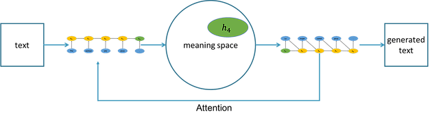
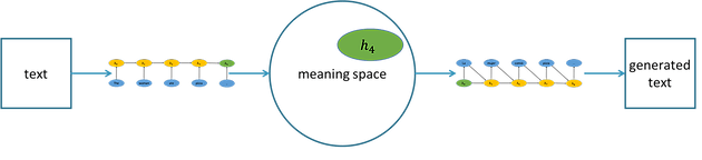
Computers are illiterate. Reading requires mapping the words on a page to shared concepts in our culture and commonsense understanding, and writing requires mapping those shared concepts into other words on a page. We currently don’t know how to endow computers with a conceptual system rich enough to represent even what a small child knows, but the field of AI has recently developed a method that can both encode representations of our world to a space of meanings (proto-read) and can transcribe points in that meaning space into language (proto-write). The method uses neural networks, so we call it neural text generation.
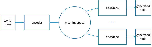
The figure above depicts neural text generation. The world state is a representation, such as an image or written sentence. The encoder is a neural network that maps the representation into a meaning space. This meaning space is a space of vectors, like the popular word vectors. These vectors are long sequences of numbers, and the space is like the familiar two-dimensional space with x and y coordinates, with the exception that there are hundreds of coordinates instead of just two. The decoders are neural networks, and there can be multiple decoders, each capable of writing a version of the meaning in a particular language or style.
Neural text generation has many uses. It is the state-of-the-art method for machine translation, where the world state consists of a sentence in a source language, which is encoded into meaning space and then decoded into one or more target languages. Neural text generation can also be useful for chatbots, where a line of dialog is encoded into a meaning space and the decoder maps that point in meaning space into a reasonable response. The method is also used for image captioning, where an image is encoded into the meaning space and then decoded into a caption. The meaning space can also be decoded into various styles of writing. Imagine having your website be dynamically customized to match the preferences and language patterns of the user. Even better, imagine being able to have your boring HR manual translated into the style of Cormac McCarthy. Something like, “The coffee in the break room is available to all employees, like some primordial soup handed out to the huddled and wasted damned.”
Neural text generation, while useful, is currently limited by a lack of common sense. It is often imprecise; if you ask a personal assistant to make you a reservation on Tuesday, it may make the appointment on Wednesday because, you know, the word vectors are pretty close (also see [51]). Neural text generation also makes mistakes that no human would make. For example, in image captioning it can mistake a toothbrush for a baseball bat [32]. But the beautiful thing is that our neural networks are getting richer, and they can show flexibility and learn from large amounts of data. As the meaning space gets closer to being able to represent the concepts that a small child can understand, we will get closer to human-level literacy. We are taking baby steps toward real intelligence.
This blog post will present an overview of neural text generation. We will start with sequence-to-sequence models, which encode source sentences and convert them to target sentences, as is done for language translation. We will then discuss the space these sentences are mapped to and how we can ensure that it is well organized, and how we can move around within this meaning space. Then we will discuss neural text generation when we don’t have pairs of sentences to train from. This will take us into generative adversarial networks (GANs) where a text generator and a classifier train each other in a virtuous arms race. We will also discuss how reinforcement learning (RL), an idea stemming from behaviorism in psychology and the training of circus animals, can be used to teach a machine how to generate useful text. Finally, we will conclude with some suggestions on when it is good to use neural text generation compared with traditional template-based generation, and we will discuss some challenges when using neural text generation.
Sequence-to-Sequence Models: Learning from Pairs of Sentences
Seq2Seq Overview
A sequence-to-sequence (seq2seq) model consists of an encoder and a decoder, and it converts one sequence of words into another. The encoder converts the source sequence of words into a vector in meaning space, and the decoder converts that vector into the target sequence of words. Both the encoder and decoder are often recurrent neural networks (RNNs). The initial big application for seq2seq models was machine translation. For example, a model can be trained to convert source sentences in English into target sentences in Spanish.
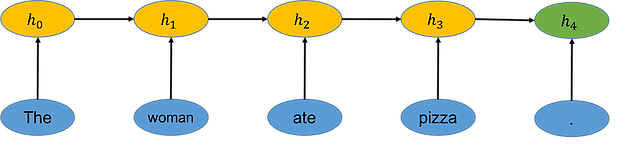
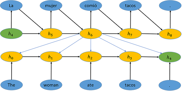
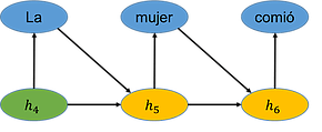
We see a depiction of the encoding process in the figure below. As each word is examined, the encoder RNN integrates it into the hidden state vector h. The vector h4 is the final state vector and contains the information in the encoded sentence. The vector h4 represents a point in the meaning space of possible meanings.
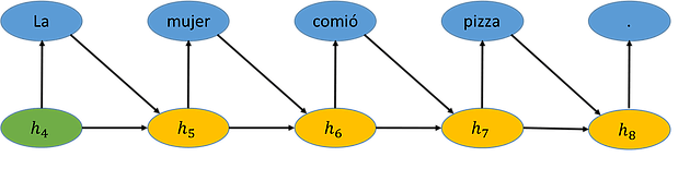
Now consider the task of decoding the sentence in the figure above into Spanish, as is shown below. We start with state h4 from the encoded sentence. We use the decoder RNN to generate the first word “La” and then the decoder uses the previous state and the last generated word to update its state to h5. It keeps doing this until it generates a stop symbol. Importantly, the number of words in the target sentence doesn’t have to be the same as the number of words in the source sentence. It stops when it generates the stop symbol, which in this case is a period.
We now see the whole seq2seq process in the figure below, with the final vector h4 of the encoding in meaning space.
Encoders
Let’s take a closer look at the encoder and how it iteratively integrates the words in a sentence into the hidden state h. In seq2seq models, words are represented as vectors stored in a vocabulary table, which represents each word in the vocabulary by a vector of a fixed dimension, such as 300. In the simplest case, we have a fixed number of words in our vocabulary, such as 50,000. We therefore have a vocabulary table of size [50,000 x 300] as shown below.
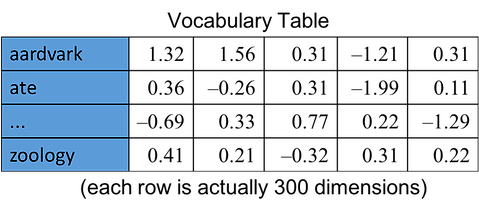
The vectors in this vocabulary table are learned as part of model training, and it results in word vectors, similar to those learned with word2vec [34]. It is worth noting that instead of using words as tokens, we can also break words into segments and use those instead. For example, the word “abomination” might be represented as the three tokens, abom@@, in@@, and ation. Here, the “@@” indicates that this word is not finished yet. The advantage of using word segments instead of whole words is that you no longer have this problem of words not being in the vocabulary. If you cut your vocabulary off at 50,000, there will still be words not in there, like maybe “abomination,” and you would be forced to replace it with a special token indicating an unknown word, such as “UNK.” There is code [45] that automatically finds good ways to split up words so that the most common words are still represented as whole words and only uncommon ones are split up at their joints.
We’ve talked about how words are represented in the vocabulary table, now let’s take a closer look at how they can be integrated into the current state of the encoder. Each cell (yellow oval in the figures) is actually a neural network with a fixed set of weights (also called parameters), and each cell in the encoder is the same neural network with the same weights. The output of the cell feeds back into the cell, that’s why it’s called recurrent. In these figures, I’ve unrolled it for easy viewing. The simplest version of a RNN cell is shown below, with the last bullet point giving the equation to generate the cell state.
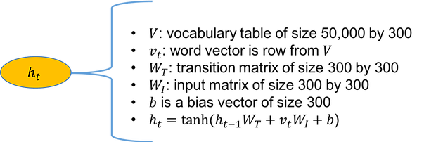
(Note that this is a simple cell to give you a grounded understanding. Most networks use more sophisticated LSTM or GRU cells, as discussed here [22].)
We can see that to update state vector h2, the vector for “ate” and the vector for h1 would be incorporated into the cell. And at h4, the output is the encoding of the sentence. The weights of the vocabulary table and RNN cell start off random and are updated through backpropagation, as discussed later.
Decoders
An RNN decoder unrolls a vector from meaning space into a target sentence. A simple decoder cell is shown below.
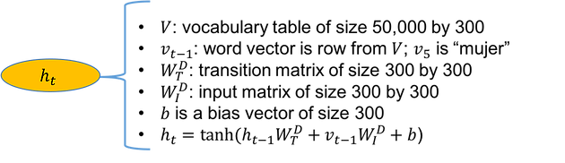
The decoder generates a probability distribution over words to write at each time step, in addition to generating the next state. In the simplest case, the output is generated by multiplying the state h by an output matrix of size [300 x 50000]. The product is a vector of size 50,000 that can be normalized into a probability distribution over words (or word segments) in the vocabulary. The network can then choose the word with the highest probability.
How can we use a corpus of paired sentences to train the encoder and decoder? The simplest way is to use a method called teacher forcing. Teacher forcing takes advantage of the fact that we know what the correct word should be because we have corresponding pairs of sentences. For example, we have a huge list of sentences in English with their Spanish translations. For our current example, at time t=6 we know that the correct word is “comió”. The cost (error) then is the negative log of the probability of the network at step 6 generating the word “comió.” Even if the network erroneously assigns a higher probability to another word, “comió” is still fed to the cell at time step 7 (the “forcing” of teacher forcing.) Now that we have a way of computing the cost (error) for a network, we can do backpropagation to train it. The backpropagation algorithm uses calculus and dynamic programming to update all of the weights in our network. The weight updates go back through the decoder cell activations into the encoder cell activations and even into the vocabulary table. Implementing backpropagation can be tricky. Luckily, tools like TensorFlow and PyTorch can do that for us.
Once the network is trained, we want to use it to generate translations for sentences it has never seen before. This is sometimes called inference. When you are actually using the model to generate text, you don’t know what the right answer is. You could take the greedy approach and always take the most likely word at each time step, but this can lead to suboptimal results. Alternatively, you could generate all sequences of words up to a given length and take the one with the lowest overall cost, but there are too many possibilities to consider. A middle ground is to use a method called beam search. You start generating with the first word, and you keep the 10 most promising sequences of words (beams) around and generate on top of those. The sentences generated by beam search can sometimes lack diversity, and there have been proposals to address this, see [23] and [24].
Attention
Notice in the encoder and decoder that the size of the state vector h stays the same even as more words are processed in the sentence. This feels counterintuitive, and it seems like some information would have to be lost. This is true. One way to get around this limitation is to use attention [25], as shown in the figure below.
At time step 6, when the network is deciding what to write, attention allows it to not just look at state h5 and the last word written but also all of the previous encoded states. It takes a weighted average of their vectors, where the weights are determined by the neural network, and it uses that weighted-average vector as additional information. The way that attention fits into the general seq2seq model is shown below.
Attention works really well. In fact, there is a seq2seq model that uses nothing but attention, see [26] and the code [27].
Applications of Seq2seq Models
Seq2seq models work on all kinds of sentence pairs. For example, you can take a bunch of dialogs and use machine learning to predict what the next statement will be given the last statement. One can mine Twitter for these dialogs, or use movie and TV subtitles [28] or dialogs of people wanting technical support [29]. Another example is text summarization [30], for example, to learn to generate headlines for news articles by using the body of the article as the source and the headline as the target. Seq2seq models can also work for style transfer. In [1], they had Mechanical Turk workers write different styles of sentences for training, upon which they applied the model.
The methodology can even be generalized and applied to image captioning. If we replace the RNN encoder on a sequence of words with a convolutional neural network (CNN) encoder on an image, everything else works the same. This assumes you have a lot of pictures with captions. See [32] and [33] for examples, and see the figure below for a depiction.

The takeaway for seq2seq models is that they work well if you have a lot of parallel sentences and you aren’t too worried about exactly what the model writes. This technology is pretty well established, and there are many implementations, such as the one in TensorFlow [37]. We will next look at the meaning space to see how it can be controlled and enriched, and later we will talk about how to reduce the reliance on parallel sentences.
Meaning Space
The meaning space is a mapping of concepts and ideas that we may want to express to points in a continuous, high-dimensional grid.
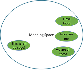
The Meaning Space Should be Smooth
We want to be able to navigate this space to generate text with the decoder, so we want the meaning space to be smooth so that points near each other in space have similar meanings, like we see with the taco-related statements in the figure below.
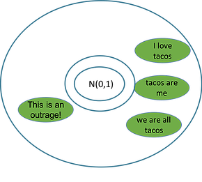
If we don’t care about the representation and are only interested in a basic application such as machine translation, we can simply let the meaning space consist of the last state of the encoder RNN. However, if we want to use the space as a representation for meaning, such as by using it with multiple decoders for multiple languages or styles, we can get more continuity in the space if we use a bias to encourage the neural network to represent the space compactly [38].
We can achieve this bias by adding an organizational constraint in the form of a prior probability distribution. The prior wants to put all points at (0,0,…,0) unless there is a good reason not to, and that “good reason” is the meaning we want to capture. By forcing the system to maintain that balance, we encourage it to organize such that concepts that are near each other in space have similar meanings. In its most basic form, this means that instead of taking the last state as it comes from the RNN, we add two dense neural network layers to the end of the encoder to convert that last state to a mean vector and a covariance vector of a multivariate normal distribution. It’s neat how neural networks and probability theory can interface in this way, and we do this conversion so that it balances the prior and the desire to represent the meaning, as we will see now.
Variational Encoding Ensures Smoothness
This balance of the prior and the meaning is achieved using something called the variational method. In the movie Arrival, variational principles in physics allowed one to know the future. We won’t cover that in this blog post, but in our world, variational methods come from the calculus of variations, which is optimization over a space of functions. Variational inference is coming up with a simpler function that closely approximates the true function.
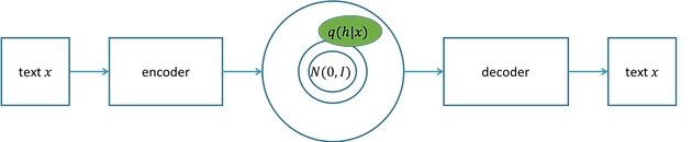
Recall that we add two dense network layers to convert the last state of the encoder into a mean vector and a variance vector of a multivariate normal distribution. This is the encoding part of what is called a variational encoder. Ideally, we want to encode text x into a meaning space representing the conditional probability distribution p(h|x), but it is hard to represent p(h|x) directly. A variational encoder approximates p(h|x) with a function q(h|x), where q(h|x) can be the multivariate normal distribution we are talking about. Since a multivariate normal distribution can be represented with a mean vector and a covariance vector (for the diagonal), all we have to do is what we said before, add these two layers on the end of our encoder that output the mean vector and covariance vector.
To maximize this approximation so that q(h|x) is as close as possible to the ideal p(h|x), it turns out that we maximize something called the (ELBO), and we use something called the reparameterization trick to keep it differentiable [39]. Part of the ELBO (shown below) is the prior p(h)=N(0,I), which forces the algorithm to use the space efficiently, which forces it to put semantically similar latent representations together. That’s the KL part in the equation, which stands for for Kullback–Leibler divergence.

Without this prior, the algorithm could put h values anywhere in the latent space that it wanted, willy-nilly. Our modified meaning space with the prior represented by the multivariate normal distribution N(0,I) is shown below.
We train the variational encoder as an autoencoder, depicted below. We encode x into the distribution q(h|x) and then sample h from q(h|x) and then pass that sample h to the decoder to regenerate x. Since we are regenerating x, it is called an autoencoder. The prior acts like regularization, so in training we are maximizing the ability of the autoencoder to reconstruct the input x, represented by p(x|h), and we are simultaneously minimizing the difference of the encoded distribution q(h|x) of x in meaning space from the 0 vector of the prior p(h), represented by the KL part. The equation is written using the expected value E.
This variational transformation of the space is not always used because it is hard to train so that the balance is right [38], but it is particularly useful if you want to measure the similarity of two blocks of text or interpolate between sentences [38].
Navigating the Meaning Space
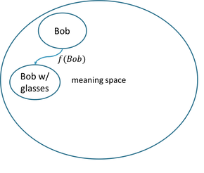
To directly control the text we generate, we need to be able to find desired parts of the meaning space. In the vision domain, Google [42] has shown how you can take an image of a face and add glasses to it or make it older, depicted in the figure below.
In the text domain, [41] provides a way to rewrite sentences to change them according to some function, such as making the sentiment more positive or making a Shakespearean sentence sound more modern. For a sentence s you want to change, the algorithm encodes it using a variational autoencoder to get h. It then looks around the meaning space to find the nearby point h* that maximizes your evaluation function. It then decodes h* to create a modified version of sentence s.
Representing and manipulating ideas in meaning space is fascinating. You could imagine a moviegoer saying, “This movie is good, but make it a little more steampunk.” Hopefully, we will start to encode and decode just about anything. The meaning space could be drawings [54] or even a space of computer programs as shown in [43] and [44]. Search in meaning space could replace searches in much larger, unorganized spaces, and since the space is smooth, we might be able to hill climb to get just about any digital artifact we wanted.
Moving Beyond Pairs of Sentences
The seq2seq model works well when you have a lot of paired training data, such as data paired with itself like in the autoencoder, or English sentences paired with their Spanish translations, or one style paired with the same content in another style, or even images with captions. We now turn our attention to methods that remove this restriction of paired data. We will discuss methods that have the different domains share encoders and bootstrap learning by using autoencoders and round-trip translations. We will also look at methods that train the algorithm to generate desired text using classifiers, including adversarial approaches. And finally, we will discuss using reinforcement learning for training our text generation algorithms.
Bridging Meanings Through a Shared Space
Consider the case where you have pairs of languages or styles but not the pairs you want. For example, you may have a lot of translations from English to Spanish and from English to Tagalog, but you want to translate directly from Spanish to Tagalog. Google faced this scenario with language translation [8]. They had data for a lot of language pairs, but they didn’t have a lot of data for all possible pairs. Their solution is depicted in the figure below.
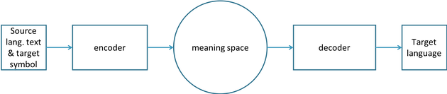
They use a single encoder and decoder for all languages. Instead of whole words, they use word segments so the encoder can use a single vocabulary table to encode all languages to the same space. They add the target language as the first symbol of the source text, so the decoder knows the language to use. After training many pairs of languages, they found they could translate pairs of languages even for which there was no paired data. The shared encoder and decoder had aligned the meaning space across languages.
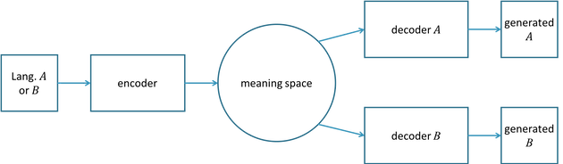
What about when you have no language pairs at all? For example, imagine you have text written in two styles, but it is not tied together in pairs. With each language or style, you can learn a language model, as depicted below.

A language model computes the probability distribution over the next word given the previous words. For the sentence, “I went to the w” it computes a probability distribution over all 50,000 words (or word segments) so the probability that word w is “store” is higher than the probability that the word w is “junkyard,” which in turn is higher than “taco.” (Incidentally, language models are the technology behind those funny blog posts of the form: “I forced my computer to watch 10,000 hours of Hee Haw and this was the result.”) In a language model, the sequence of words has to start somewhere. How does it know the probability distribution of the first word? The decoder needs to be associated with a meaning space.
The way to associate text with a meaning space is to train it as an autoencoder. This is the same autoencoder that we encountered previously. The question then becomes how to align up the meaning spaces of the different languages or styles so that one can translate between them. One way to align the meaning spaces is to ensure that the autoencoders of the different languages or styles use the same encoder [7]. This results in the model depicted below.
With this model, we can create synthetic pairs for training. Creating synthetic pairs means that we create the aligned pairs and then train the model as a regular seq2seq model using those synthetic pairs as training data. For example, to map language A to B, we could encode sentences in B and then decode them with the decoder for A, and then we would have pairs of the form (A, B). You start with a sentence in B because we want to do our training in the other direction, starting from sentences in A. To create pairs of the form (B, A), we start with A. In general, this method of creating pairs is called back-translation [13].
Instead of explicitly creating synthetic pairs, we can use the cost of a round-trip translation as a training signal. For example, we can translate a sentence in A to a sentence in B and then translate that sentence in B back into language A, and we can use the cost of translating that sentence in B to language A for training both the shared encoder and the decoder of A. This was done by [6] for text attribute transfer, for example for converting a text from positive to negative sentiment. For instance, for a Yelp review, they automatically converted the positive sentiment phrase “love the southwestern burger” to the negative sentiment phrase “avoid the grease burger.” Notice that the word “burger” is in both, as it should be. Maintaining semantic meaning can sometimes be a challenge with these systems. In their work [6], they add an additional constraint that nouns should be maintained.
The language translation system from Microsoft [9] uses similar principles to achieve human-level performance on translating Chinese to English. They have pairs between these languages, but by using a method called dual learning, they can leverage additional monolingual training data. In dual learning [12], there is a model from language A to language B and a model from language B to language A that are trained together. Dual learning also entails training language models on A and B individually. Then, it seeks to maximize the communication reward, which is the fidelity of a round-trip translation of a sentence in A to language B and then back back to language A (and B to A and back to B), and also to maximize the language model reward, which for A to B is how likely the sentence in B is in the monolingual language model for B (and likewise for B to A). Instead of using teacher forcing, dual learning uses policy gradient, which will be discussed shortly.
Adversarial Text Generation
We have looked at aligning meaning spaces using autoencoders and round-trip training; another approach to training our algorithm to generate text without aligned pairs of sentences is to use supervised classification on the entire generated sentence. Supervised classification means that we train a learning algorithm to predict labels by feeding it a bunch of records where we already know the label. For example, we could train a classifier to predict who will repay a loan by feeding it records from the past, each labeled with whether the person repaid the loan. We have already used supervised classification at the word level with teacher forcing, and we now look at training a classifier to determine whether our generated text on the whole has a desired property. By doing this, our text generation algorithm can seek to generate text that will be classified as having that desired property.
The method [14] depicted in the figure below runs a classifier (also called a discriminator) on top of generated text. They encode text using a variational autoencoder and add an additional label (feature) in the encoding that is used by the decoder when decoding. Then, the classifier on the other side of the decoder determines whether the decoded text has the proper label. The dotted line indicates learning signal feeding backward from the classifier.
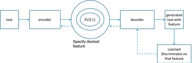
They showed how one could generate negative past-tense sentences such as “the acting was kind of hit or miss” and positive present-tense sentences such as “this is one of the better dance films” by specifying those labels (features) in meaning space. And they showed how one could convert the tense of a particular sentence by changing that label in the meaning space. By doing this, the sentence “this was one of the outstanding thrillers of the last decade” was converted to “this will be one of the great thrillers of the all time.”
We can also consider classifiers (often called discriminators) as part of a general framework called Generative Adversarial Networks (GANs) [11], as depicted below.

GANs consist of a generator and a discriminator (classifier). The generator takes a random seed and from that creates digital artifacts (synthetic data) such as images or sentences. The discriminator then tries to tell the difference between the synthetic data and real examples of that data. The results of the discriminator can serve as the error value for the generator, so that if the discriminator can easily tell the real data from the synthetic data, the error for the generator is high. In continuous domains like images, we can use this error for backpropagation to make the generator better. As the generator gets better, the discriminator has to get better at telling real from generated, so you have a virtuous cycle. In the vision domain, the results are astounding: a generator can create synthetic images of people that look just like real people, but they don’t exist.
In the text domain, we can’t as easily use this error from the discriminator because we have to pick discrete words instead of being able to change continuous pixel values. Picking discrete words in sequence means that the algorithm is not differentiable and so we can’t do backpropagation. There are three methods to deal with this lack of differentiability. The first method is to not pick specific words at each time step and instead to use the weighted average of the word vectors, where the weights come from the output word probability distribution of each cell of the decoder. This is what was done in the classifier method [14] we saw previously. The second method is to use reinforcement learning, which we will describe in the next section. The third method is to apply the discriminator to the continuous meaning space or to the continuous space of hidden states generated by the decoder.
One such method of applying a discriminator to the continuous hidden states of a decoder is called professor forcing [15]. In professor forcing, the discriminator of the GAN focuses on telling the difference between hidden states when the decoder is running in teacher forcing mode and running in inference mode. The original goal of this work was not to transfer style or language, but rather to make the decoder better at decoding when it gets off track and starts generating sequences that are significantly different from the training data. In [5], they use professor forcing for style transfer. They encode a sentence in a source style and they use a discriminator to ensure the hidden states of the decoding of that sentence are close to the hidden states of a normal sentence in the target style.
Learning Through Reinforcement Learning
Reinforcement learning (RL) is an alternative to teacher forcing for training our text generation algorithm. Reinforcement learning is a gradual stamping in of behavior that comes from receiving rewards and punishments (negative rewards). RL was studied in animals by Thorndike [48] as far back as 1898, and it later became the study of behaviorism in psychology [47]. It was then formulated into artificial intelligence; see the leading book by Sutton and Barto [16].
When using reinforcement learning for neural text generation, the actions are writing words and the states are the words the algorithm has already written. Choosing the best word to write is hard because there are as many actions as there are words in your vocabulary, usually around 50,000. A kind of reinforcement learning that works well in domains with large action spaces is called policy gradient (see [17] and [18]). A policy specifies what action to take (in our case what word to write) for each state. Policy gradient methods learn a policy directly on top of a neural network; basically, they learn which action to take as a classification problem [18]. This means that reinforcement learning starts to look more like supervised learning, where the labels are actions. Instead of doing gradient descent on the error function as in supervised learning, you are doing gradient ascent on the expected reward. Each action you take is the “correct” label for the current state, and the loss for that correct label is scaled by whether that action turned out to be good or bad, meaning, roughly, whether you got a positive or negative reward.
When using GANs, this reward will come from the discriminator, and so the discriminator determines the policy gradient. For example, this discriminator could try to tell the difference between dialog responses created by humans and ones created by the generator, and the generator would receive a positive reward when it can fool the discriminator, as was done in [3].
One difficulty with these high dimensional spaces is that it is hard to learn what action to take now (what word to write) when you don’t get a reward until much later when the discriminator is run and the sentence is scored. To address this problem, we can use either Monte Carlo search or the actor-critic method.
In Monte Carlo search, the algorithm does a search forward from the current state to the end to estimate how good different actions are at the current time step. For example, in the figure below, if we were to write “comió” and follow our current policy after that, how good would the final reward be?
We can use the estimate created by searching (simulating) forward until the end as the current reward now, as was done in [59]. That “how good” is the estimate we use to determine whether writing “comió” should be the action this network takes in the future when in a similar state. This approach is also used in game-playing AI, for example with the recent success in the game Go [20].
In actor-critic methods, instead of searching forward to determine how good each action might be in the current state, or how good the current state is, you have another neural network that learns to estimate the value of each state or state-and-action pair directly. This neural network is called the critic [17]. An example GAN for text that uses this approach is MaskGAN [21] (code available here [36]).
Currently, GANs have some drawbacks for text generation. The first is mode collapse: once the generator figures out how to fool the discriminator, it may keep generating the same thing over and over again. The second drawback is that GANs are hard to train because it is difficult to keep the generator and discriminator in balance. The third drawback is that training is slow. If your vocabulary size is 50,000, the algorithm has to try 50,000 random actions in many states. To reduce this search, researchers often pre-train text GANs with teacher forcing so that the generator chooses sequences of words during training that are at least reasonable. For a survey of reinforcement learning for generating text, see [2], and see [4] for an example of semi-recent work. Also, see the code implementations at [35].
The application of deep learning to reinforcement learning is still a work in progress [46]. Before deep learning, one significant challenge to employing reinforcement learning was abstracting the state. The world is complicated, and the only way to learn is to know when states are similar to states the algorithm has seen before. In 2013, [56] made a significant breakthrough using deep learning to play Atari with Deep Q-Networks (DQN). The input was the direct video from the game, and they used deep learning to solve the state abstraction problem. That algorithm couldn’t think very far ahead, but there has been significant recent progress in playing complicated video games, such as Dota 2 [58], capture the flag [57], and Doom [55]. Text generation has a larger set of possible actions than most video games because it requires choosing among which of 50,000 words to write at each time step, but these games are complex as well, and we can expect that many of these advancements will begin making their way into text generation.
Conclusion
When should you use neural text generation? If you can enumerate all of the patterns for the things you want the computer to understand and say, use context-free grammars for understanding [49] and templates for language generation [10]. You could, for example, build a chatbot where you use machine learning to map the input text to different possible topics where you have a context-free grammar for each topic. Another example is writing stories for Little League baseball games [52]. If you can come up with a couple dozen ways that a baseball game can go, pitchers duel, slugfest, come-from-behind victory, you can take the stats from the game and use it mad-libs style to automatically write a story.
If, on the other hand, you can’t enumerate all of the things you want the computer to understand and say, but you have a lot of data, neural text generation might be the way to go. Machine translation, of course, is an ideal example. Neural text generation is also useful if you want to convert between styles. What neural text generation lacks is exactness. Most of the time, we want our machines to say exactly what we mean them to say. We don’t want our website to tell people that all printing presses are 50% off when we intended the sale to be for inkjet printers.
Adding symbolic exactness back into the meaning space is a pressing problem. There has been some work in this direction, for example in generated summaries [53]. As we saw in [6], the scoring of style transfer can include whether nouns were preserved during translation of one style to another. Another option is pointer networks, which can choose to copy specific information from the source text during the decoding [50]. In addition to lacking exactness, neural text generation doesn’t yet work well on long text, but the attention-based method [26] seems promising in this regard.
Machines will be illiterate for a long time, but as algorithms get better at controlling and navigating the meaning space, neural text generation has the potential to be transformative. Few things are more enjoyable than reading a story by your favorite author, and if we could have all of our information given to us in a style tailored to our tastes, the world could be enchanting.
References
-
Seq2seq style transfer: Dear Sir or Madam, May I introduce the YAFC Corpus: Corpus, Benchmarks and Metrics for Formality Style Transfer, https://arxiv.org/pdf/1803.06535.pdf
-
Neural Text Generation: Past, Present and Beyond, https://arxiv.org/pdf/1803.07133.pdf
-
Adversarial Learning for Neural Dialogue Generation, https://arxiv.org/pdf/1701.06547.pdf
-
Actor-Critic based Training Framework for Abstractive Summarization, https://arxiv.org/pdf/1803.11070.pdf
-
Style Transfer from Non-Parallel Text by Cross-Alignment, https://arxiv.org/pdf/1705.09655.pdf
-
Improved Neural Text Attribute Transfer with Non-parallel Data, https://arxiv.org/pdf/1711.09395.pdf
-
Unsupervised Neural Machine Translation, https://arxiv.org/pdf/1710.11041.pdf
-
Zero-Shot Translation with Google’s Multilingual Neural Machine Translation System, https://research.googleblog.com/2016/11/zero-shot-translation-with-googles.html
-
Achieving Human Parity on Automatic Chinese to English News Translation, https://arxiv.org/pdf/1803.05567.pdf
-
Summer School on Natural Language Generation, Summarisation, and Dialogue Systems, http://nlgsummer.github.io/index.html
-
Ian J. Goodfellow, Jean Pouget-Abadie, Mehdi Mirza, Bing Xu, David Warde-Farley, Sherjil Ozair, Aaron Courville, Yoshua Bengio, Generative Adversarial Networks, https://arxiv.org/abs/1406.2661.
-
Dual Learning for Machine Translation, https://papers.nips.cc/paper/6469-dual-learning-for-machine-translation.pdf
-
Improving Neural Machine Translation Models with Monolingual Data, http://www.aclweb.org/anthology/P16-1009
-
Toward Controllable Text Generation, https://arxiv.org/pdf/1703.00955.pdf
-
Professor Forcing: A New Algorithm for Training Recurrent Networks, https://arxiv.org/pdf/1610.09038.pdf
-
Reinforcement Learning: An Introduction. See new book online http://incompleteideas.net/book/bookdraft2018jan1.pdf
-
D. Silver, http://www0.cs.ucl.ac.uk/staff/d.silver/web/Teaching_files/pg.pdf
-
Deep Reinforcement Learning: Pong from Pixels, http://karpathy.github.io/2016/05/31/rl/
-
SeqGAN: Sequence Generative Adversarial Nets with Policy Gradient, https://arxiv.org/pdf/1609.05473v3.pdf
-
Mastering Chess and Shogi by Self-Play with a General Reinforcement Learning Algorithm, https://arxiv.org/pdf/1712.01815.pdf
-
MaskGAN: Better Text Generation via Filling in the Blank, https://arxiv.org/pdf/1801.07736.pdf
-
Understanding LSTM Networks, http://colah.github.io/posts/2015-08-Understanding-LSTMs/
-
Mutual Information and Diverse Decoding Improve Neural Machine Translation, https://arxiv.org/pdf/1601.00372v2.pdf
-
Diverse Beam Search: Decoding Diverse Solutions from Neural Sequence Models, https://arxiv.org/pdf/1610.02424v1.pdf
-
Neural Machine Translation by Jointly Learning to Align and Translate, https://arxiv.org/abs/1409.0473
-
Attention Is All You Need, https://arxiv.org/abs/1706.03762
-
Tensor2tensor code https://github.com/tensorflow/tensor2tensor
-
OpenSubtitles, http://opus.lingfil.uu.se/OpenSubtitles.php
-
The Ubuntu Dialogue Corpus: A Large Dataset for Research in Unstructured Multi-Turn Dialogue Systems, https://arxiv.org/abs/1506.08909
-
Deep Learning for Text Summarization, https://memkite.com/deeplearningkit/2016/04/23/deep-learning-for-text-summarization/
-
Seq2seq style transfer: Dear Sir or Madam, May I introduce the YAFC Corpus: Corpus, Benchmarks and Metrics for Formality Style Transfer https://arxiv.org/pdf/1803.06535.pdf
-
Deep Visual-Semantic Alignments for Generating Image Descriptions, http://cs.stanford.edu/people/karpathy/deepimagesent/
-
A picture is worth a thousand (coherent) words: building a natural description of images, http://googleresearch.blogspot.com/2014/11/a-picture-is-worth-thousand-coherent.html
-
TensorFlow word2vec tutorial, https://www.tensorflow.org/tutorials/word2vec
-
Texygen code https://github.com/geek-ai/Texygen
-
MaskGAN code https://github.com/tensorflow/models/tree/master/research/maskgan
-
Neural Machine Translation (seq2seq) Tutorial, https://github.com/tensorflow/nmt
-
Generating Sentences from a Continuous Space, https://arxiv.org/abs/1511.06349
-
Auto-Encoding Variational Bayes, https://arxiv.org/pdf/1312.6114.pdf
-
Variational Autoencoder in TensorFlow, https://jmetzen.github.io/2015-11-27/vae.html
-
Sequence to Better Sequence: Continuous Revision of Combinatorial Structures, http://www.mit.edu/~jonasm/info/Seq2betterSeq.pdf
-
Latent Constraints: Learning to Generate Conditionally from Unconditional Generative Models, https://arxiv.org/pdf/1711.05772.pdf
-
Neural Symbolic Machines: Learning Semantic Parsers on Freebase with Weak Supervision, https://arxiv.org/pdf/1611.00020.pdf
-
Learning to Organize Knowledge with N-Gram Machines, https://arxiv.org/pdf/1711.06744.pdf
-
Subword Neural Machine Translation, https://github.com/rsennrich/subword-nmt
-
Deep Reinforcement Learning Doesn’t Work Yet, https://www.alexirpan.com/2018/02/14/rl-hard.html
-
Skinner, B. F. Science and human behavior, Simon and Schuster, 1953
-
Thorndike, E., Animal intelligence: an experimental study of the associative processes in animals, Columbia University, 1898
-
Chatbots: Theory and Practice, https://medium.com/intuitionmachine/chatbots-theory-and-practice-3274f7e6d648
-
Pointing the Unknown Words, http://www.aclweb.org/anthology/P16-1014
-
A Random Walk Through EMNLP 2017, http://approximatelycorrect.com/2017/09/26/a-random-walk-through-emnlp-2017/
-
Parents Pay for Little League Sports Recaps Written by Computers, https://abcnews.go.com/Business/parents-pay-league-sports-recaps-written-computers/story?id=34743643
-
Faithful to the Original: Fact Aware Neural Abstractive Summarization, https://arxiv.org/pdf/1711.04434.pdf
-
A Neural Representation of Sketch Drawings, https://arxiv.org/pdf/1704.03477.pdf
-
World Models, https://worldmodels.github.io/
-
Playing Atari with Deep Reinforcement Learning, https://arxiv.org/pdf/1312.5602.pdf
-
Capture the Flag: the emergence of complex cooperative agents, https://deepmind.com/blog/capture-the-flag/
-
OpenAI Five, https://blog.openai.com/openai-five/
-
SeqGAN: Sequence Generative Adversarial Nets with Policy Gradient, https://arxiv.org/pdf/1609.05473v3.pdf
Hi, this is a comment.
To get started with moderating, editing, and deleting comments, please visit the Comments screen in the dashboard.
Commenter avatars come from Gravatar.