
Reinforcement learning (RL) is an effective method for solving problems that require agents to learn the best way to act in complex environments. RLlib is a powerful tool for applying reinforcement learning to problems where there are multiple agents or when agents must take on multiple roles. There are many of resources for learning about RLlib from a theoretical or academic perspective, but there is a lack of materials for learning how to use RLlib to solve your own practical problems. This tutorial helps to fill that gap.
120 Years of Reinforcement Learning
We first fly through 120 years of reinforcement learning work. If you want to get right into RLlib, fell free to skip to the next section.
Thorndike observed that some behaviors in animals arise from a gradual stamping in [Thorndike, 1898]. In psychology, this stamping in became the study of Behaviorism [Skinner, 1953] (see the Skinner box Figure 1). Behaviorism was the dominant paradigm for investigating human psychology and learning in the middle of the 20th century. It focused only on the responses that could be observed and studied the different conditions and training regimens that led to those responses. It was popular because it wasn’t’ fluffy—you could make testable predictions. The behaviorism framework proved too limiting to describe human psychology, but it showed itself to be a useful formulation for learning in artificial agents such as robots [Sutton and Barto, 1998], where it is called “reinforcement learning” (often abbreviated as RL).

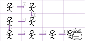
At its simplest, in reinforcement learning an agent begins by randomly exploring until it reaches its goal, as depicted in Figure 2.
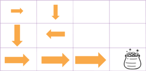
When it reaches the goal, credit is propagated back to its previous states, as depicted in Figure 3. The agent learns a function Q(s,a), which gives the cumulative expected discounted reward of being in state s and taking action a and acting according to the current policy thereafter. The values of Q(s,a) are depicted as the size of the arrows in Figure 3.
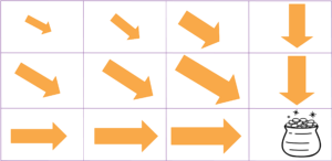
The agent starts out with a policy of just taking random actions. The policy is continually updated from experience, and eventually the agent learns the value of being in each state and taking each action and can therefore always do the best thing in each state. This behavior is then represented as a final policy, as depicted in Figure 4.
In the examples in the previous figures there was a discrete state and action space. This discrete state space is limiting because as the number of variables that makes up your state grows the size of the space grows exponentially. This means that you can’t visit all possible states, much less visit each one enough to learn Q(s,a). Because of this limitation, modern RL uses neural networks, as depicted in Figure 5.
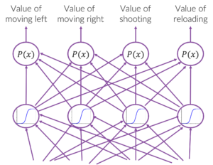
RLlib automatically constructs neural network (deep learning) models behind the scenes based on your configuration. This tutorial focuses on RLlib.
RLlib is particularly good for learning with multi-agents, such as swarms, or learning across multiple machines. If you are just looking for straightforward RL with a single agent on a single machine, I recommend starting with StableBaselines3. If you want to learn more about reinforcement learning in general, see these great resources. On to RLlib.
Overview of RLlib
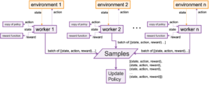
RLlib was built to solve the problem of distributed RL, as described in this paper. Parallel training in RL is hard because you must keep the policies in synch. RLlib solves this problem by using Ray. Ray is a system for parallel training, and RLlib is built on top of it. We see a depiction of parallel training in Figure 6.
Each copy of the environment can be running on a different computer. The environment is where the agent is actually acting in the world. Each worker uses a copy of the current policy to choose actions for the agent that are executed in the environment. The reward function then determines how good that resulting state is, and data samples in the form of (state, action, reward) tuples are sent to a central processor. The central processor then uses those samples to update the policy, which is broadcast out to the workers on the different machines. This policy update can be done with TensorFlow or PyTorch.
Parallel training is necessary for scaling, but for me the most exciting part of RLlib is the abstractions it provides for hierarchical multiagent reinforcement learning, and that is what we will focus on in the next couple of sections.
Hierarchical, Multi-Agent Example Environment
For this tutorial, we created a simple, custom, multi-agent, hierarchical environment to show you how to adapt RLlib to your problem. The environment and the code can be found here. Using a custom environment prevents us from glossing over any necessary details for using RLlib in your system. The environment is silly but entails the necessary complexity.
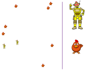
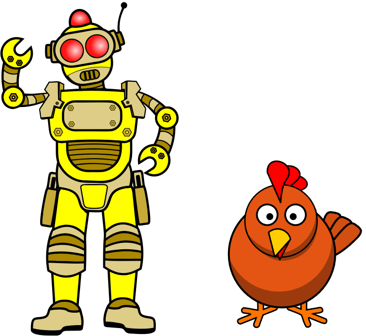
The environment of two robots in a chicken yard is shown in Figure 7. The robots want to capture (move to) the chickens that are most like them. In this scenario, each robot and each chicken has a personality based on the OCEAN model. The reward for the robots comes from getting close to a chicken that has a similar personality to the robot. The robot is also punished by life on each timestep (it receives a small negative reward per timestep), and its reward when it reaches the chicken is computed as the dot product of its personality with that of the chicken. For example, neurotic robots are more highly rewarded for finding equally neurotic chickens.
This environment is simple but it is multiagent and hierarchical. There are two robots, and each robot uses two policies:
- High-level policy: pick a chicken
- Low-level policy: move to chicken
The way the high-level policy sees the world is as a list of chickens, where each chicken’s personality is represented with a five-dimensional vector, and each chicken has an x and y location. The action space of the high-level policy is which chicken to choose.
The low-level policy is for when a chicken is already chosen, so it sees the world as the position of the robot x and y and the position of the chosen chicken, x and y. The action space of the low-level policy is to go in 8 directions: N, NE, E, SE, S, SW, W, and NW.
The episode ends when both robots get within a distance threshold of a chicken. The environment is shown in YourTargetSystem and YourAutonomousAgent in the repo. We will cover how the state and the action spaces for both policies are represented in the next section (Figure 9).
RLlib Abstractions
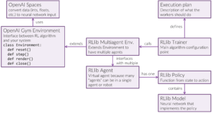
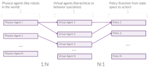
We can think of RLlib in terms of its main abstractions shown in Figure 8. We will refer to this diagram as we go through the rest of the tutorial.
OpenAI Spaces
OpenAI created a the OpenAI Gym framework for reinforcement learning a few years back. Gym provides nice abstractions that are carried forward into both StableBaselines3 and RLlib.
The first significant piece of Gym is spaces, which make it easy to format your domain for neural networks. The observation spaces of the high-level and low-level policies are from your_openai_spaces.py are shown here.
robot_position_space = spaces.Box(
            shape=(2,),
            dtype=np.float,
            low=0.0,
            high=1.0)

robot_ocean_space = spaces.Box(
            shape=(NUM_OCEAN_FEATURES,),
            dtype=np.float,
            low=0.0,
            high=1.0)

high_level_obs_space = spaces.Dict({
        'chicken_oceans': chicken_ocean_space,
        'chicken_positions': chicken_position_space,
        'robot_ocean': robot_ocean_space,
        'robot_position': robot_position_space,
})

low_level_obs_space = spaces.Dict({
        'robot_position': robot_position_space,
        'chicken_positions': chicken_position_space,
})
We see that we can represent these spaces in a semantically meaningful way. The beautiful thing about OpenAI spaces is that the learning agent can automatically translate this representation into input for a neural network.
OpenAI Gym Environment
The second significant piece of OpenAI Gym is the Env class. Env provides an uniform API to interact with your environment. We see in Figure 8 that the Env class has four main methods.
- reset
- step
- render
- close
Reset starts the episode over, render gives you an opportunity to visualize your environment, and close lets you close down.
The most important method is step. The input to the method is the action chosen by the policy. The output from the method is the observed state and the reward. The learning algorithm then uses this observation and reward to update the policy. The output for the method also includes whether the episode is done and any other important information you want to add through customization. The step method is run inside a worker in Figure 6.
I mentioned previously that I thought the most exciting part of RLlib is its abstractions for working with multiple and hierarchical agents. RLlib enables this functionality by extending OpenAI Gym Env class to work for multiple agents with the class MultiAgentEnv. In the step method of MultiAgentEnv the actions from the policies come in as a dictionary with one key for each agent name. Likewise, the information passed out is a dictionary with the units as keys (more on this later).
You control which agents are active by returning observations for only those agents, as you can see in the step function of your_rllib_environment. If an agent is not active, you don’t supply it an observation when returning from the step method. If there is no observation for an agent, then when the step function is called on the next timestep that agent won’t have an action. In this way, the RLlib MultiAgentEnv class enables you to dynamically say which of your agents are acting at which timesteps and you can specify what their observation and reward should be if they are active.
In fact, you can have multiple virtual agents per physical robot as a hierarchy of agents, as shown in Figure 9. You can also have a swarm of agents that share a policy so that anything learned by one agent in the swarm transfers to the other agents.
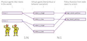
In particular, the setup for our environment is shown in Figure 10. This mapping is specified in our config file, your_rllib_config.py.
Testing Your Environment
Reinforcement learning is hard to debug. I don’t believe that life always finds a way, but RL agents will adapt to the world you give them, even if that world is not what you think it is. So a good way to start is with a random policy to test that your environment works as expected.
Initially, we factor RLlib out for testing so we can confirm that the environment works as expected, as shown in demo/demo_your_rllib_env.py and excerpted below
env = YourEnvironment(config)
env.reset()

action_dict = {'robot_1_high': random.choice(range(NUM_CHICKENS)),
                'robot_2_high': random.choice(range(NUM_CHICKENS))}

obs, rew, done, info = env.step(action_dict)
env.render()

while not is_all_done(done):
    action_dict = {}
    assert 'robot_1_low' in obs or 'robot_2_low' in obs
    if 'robot_1_low' in obs and not done['robot_1_low']:
        action_dict['robot_1_low'] = random.choice(range(NUM_DIRECTIONS))
    if 'robot_2_low' in obs and not done['robot_2_low']:
        action_dict['robot_2_low'] = random.choice(range(NUM_DIRECTIONS))
    obs, rew, done, info = env.step(action_dict)
    print("Reward: ", rew)
    time.sleep(.1)
    env.render()
The code first passes in random high-level actions, and then it loops over random low-level actions until both robots have reached a chicken. This is a useful way to see what is happening in the step function. Notice that we pass in actions only for agents (high or low) that we want to act.
Learning a Policy
To train your policy, you pick a trainer (algorithm) and tie your environment to it. RLlib comes with trainers for most of the standard algorithms, such as Proximal Policy Optimization (PPO) and Deep Q Networks (DQN). There are two ways to run your trainer as shown in your_rllib_train.py and excepted below
if RUN_WITH_TUNE:

    tune.registry.register_trainable("YourTrainer", YourTrainer)
    stop = {
            "training_iteration": NUM_ITERATIONS  # Each iter is some # of episodes
        }
    results=tune.run("YourTrainer",stop=stop,config=config,checkpoint_freq=10)

    # You can just do PPO or DQN but we wanted to show how to customize
    #results = tune.run("PPO",stop=stop,config=config,verbose=1,checkpoint_freq=10)

else:
    from your_rllib_environment import YourEnvironment
    trainer = YourTrainer(config, env=YourEnvironment)

    # You can just do PPO or DQN but we wanted to show how to customize
    #from ray.rllib.agents.ppo import PPOTrainer
    #trainer = PPOTrainer(config, env=YourEnvironment)

    trainer.train()
The first way is with Ray Tune. Ray Tune was originally developed for hyperparameter tuning, but works well for running RL algorithms. The second way is to run the trainer directly.
With Tune, the environment is specified in the config dictionary. When running it directly, you can specify the environment as a separate parameter. Regardless, configuration is a big part of the flexibility of RLlib, and it is worth taking a few minutes to go over it. The configuration is stored in a giant dictionary that comes from multiple levels of inheritance. The first level is at the general trainer level. Then, the type of trainer you use inherits it and adds to it, for example with PPO. Finally, you add to the config for your particular implementation; for example, to map agents to policies.
You can also create a custom trainer. The custom trainer is actually used in the tutorial code to demonstrate how that is done, but you can comment it out and uncomment the standard PPO trainer. A custom trainer allows you to do any operation you want through a custom execution plan. It can be a little trickly to get it all working together, but there are few limits to customization.
Looking at your training results
As shown in Figure 11, when you run your_rllib_train.py you get 83 graphs in TensorBoard.

To see these on your machine, Go to /Users/you/ray_results to find your run and type “tensorboard logdir=./”.
I let it run on my laptop for about an hour. That’s a long time for a small environment, but we didn’t add any smart features, and if you want, RLlib lets you put this directly on a cluster of machines by increasing the number of workers and turning off local mode ray.init(local_mode=False).
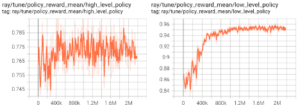
Figure 12 shows the mean policy rewards over time. The two robots share both a high-level policy and a low-level policy. The high-level policy learned at the beginning but there is a lot of randomness (evidently, finding the right chicken is hard). In Figure 12, the x-axis is timesteps, and the y-axis is reward.
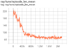
Recall that the robots are punished a small amount on every timestep. This “reward” encourages them to find chickens increasingly quickly, as shown in Figure 13. In the figure, the x-axis is timesteps, the y-axis is the number of timesteps it takes for both robots to find a chicken.
Loading and using the policies
It’s no good to train if you can’t use the policy. After the policy is learned, we can load it up and get the best action for any state in demo/demo_after_training.py. In the excerpt below we see we see how to load a trainer with saved parameters.
from your_rllib_environment import YourEnvironment
trainer = ppo.PPOTrainer(config, env=YourEnvironment)
run = 'YourTrainer_YourEnvironment_d9c79_00000_0_2022-08-18_21-37-21'
checkpoint = 'checkpoint_000500/checkpoint-500'
restore_point = os.path.join(YOUR_ROOT, run, checkpoint)
trainer.restore(restore_point)
And below we see how to call compute_single_action to get a best action from the learned policy for a current state.
robot_1_high_action = trainer.compute_single_action(obs['robot_1_high'], policy_id='high_level_policy', explore=False)
robot_2_high_action = trainer.compute_single_action(obs['robot_2_high'], policy_id='high_level_policy', explore=False)

action_dict = {'robot_1_high': robot_1_high_action,
                'robot_2_high': robot_2_high_action}

obs, rew, done, info = env.step(action_dict)

env.render()

def is_all_done(done: Dict) -> bool:
    for key, val in done.items():
        if not val:
            return False
    return True

while not is_all_done(done):
    action_dict = {}
    assert 'robot_1_low' in obs or 'robot_2_low' in obs
    if 'robot_1_low' in obs and not done['robot_1_low']:
        action_dict['robot_1_low'] = trainer.compute_single_action(obs['robot_1_low'], policy_id='low_level_policy')
    if 'robot_2_low' in obs and not done['robot_2_low']:
        action_dict['robot_2_low'] = trainer.compute_single_action(obs['robot_2_low'], policy_id='low_level_policy')
    obs, rew, done, info = env.step(action_dict)
    print("Reward: ", rew)
    env.render()
You can also look at the policy itself, as we see in demo/demo_look_at_policies.py. You can look at the actual parameters and the size of the automatically created neural network.
from your_rllib_environment import YourEnvironment
trainer = ppo.PPOTrainer(config, env=YourEnvironment)

# Change these for your run
run = 'custom_execution_plan_2022-02-24'
checkpoint = 'checkpoint_000500/checkpoint-500'

restore_point = os.path.join(YOUR_ROOT, run, checkpoint)
trainer.restore(restore_point)

print("************** high level policy **************************************")
# Note the output size of 10
policy: Policy = trainer.get_policy('high_level_policy')
# https://github.com/ray-project/ray/blob/releases/1.10.0/rllib/models/torch/complex_input_net.py
model: ComplexInputNetwork = policy.model
for m in model.variables():
    print(m.shape)

print("**************** low level policy **************************************")
# Note the output size of 8
policy: Policy = trainer.get_policy('low_level_policy')
model: ComplexInputNetwork = policy.model
for m in model.variables():
    print(m.shape)
Conclusion
RLlib is complicated but powerful. It is particularly good for training swarms of agents and for providing flexibility to do just about whatever you want. After you go through this tutorial, you can look at the repo, especially the examples, and when you get stuck you can post something on the discussion.
References
Thorndike, E. L. (1898). Animal intelligence: An experimental study of the associative processes in animals.
Skinner, B. F. (1953). Science and human behavior. Simon and Schuster.
Sutton, R. S., & Barto, A. G. (1998). Reinforcement Learning. MIT Press.
Credits
Icons from publicdomainvectors.org https://publicdomainvectors.org/
robot https://publicdomainvectors.org/en/free-clipart/Yellow-robot/81372.html